Artemis (2026) - Thermal Modeling of Battery Pack

Overview
#

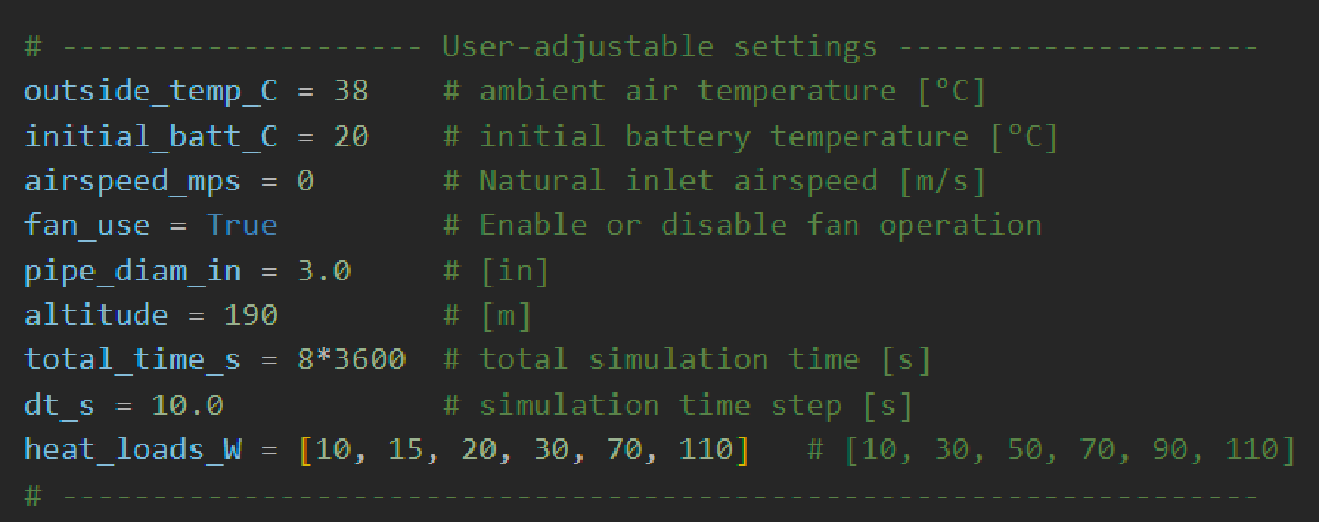
A transient thermal simulation tool for predicting battery pack temperatures under various heat loads and cooling configurations. The simulator models forced-air convection through a tube bank (cylindrical battery cells) with fan control, enabling design optimization of the cooling system for a solar racing vehicle.

Language: Python 3.12 (Using CoolProp, SymPy, NumPy, modified Tubebank libraries)

Key Features
#

Feature	Description
Transient Simulation	Time-stepping thermal model with configurable dt
Component-Based Architecture	Modular classes for Inlet, Piping, ThermalLoad, Fan, Exhaust
Real Thermophysical Properties	CoolProp library for temperature/pressure-dependent air properties
Multiple Heat Transfer Correlations	Dittus-Boelter, Sieder-Tate, Zukauskas tube bank
Lumped Capacitance Battery Model	Temperature-dependent thermal capacitance and internal resistance
Fan Curve Modeling	Symbolic pressure-flow curves with PWM duty cycle control
System Impedance Matching	Automatic fan operating point determination

System Architecture
#

┌─────────┐   ┌─────────┐   ┌─────────────┐   ┌─────┐   ┌─────────┐   ┌─────────┐
│  Inlet  │ → │  Pipe1  │ → │ ThermalLoad │ → │ Fan │ → │  Pipe2  │ → │ Exhaust │
└─────────┘   └─────────┘   │ (Battery)   │   └─────┘   └─────────┘   └─────────┘
                            └─────────────┘

Each component implements a process() method with signature:

@abstractmethod
def process(self, air_flow, air_temp, velocity, pressure, density, **kwargs):
    pressure_out = pressure
    return air_flow, air_temp, velocity, pressure_out, density

Outputs are fed in series through the defined cooling system. This allows for compartmentalization and modular testing of each component, and together as a system. Code can be written for specific parts, and improved independently. Complete systems can be swapped out or reconfigured easily in code.

Physics & Equations
#

Governing Energy Balance
#

The battery temperature evolves according to:

$$\frac{dT_{batt}}{dt} = \frac{\dot{Q}_{gen} - \dot{Q}_{conv} - \dot{Q}_{rad}}{C_{batt}(T)}$$

Where:

$\dot{Q}_{gen}$ = Internal heat generation (I²R losses)
$\dot{Q}_{conv}$ = Convective heat transfer to air
$\dot{Q}_{rad}$ = Radiative heat transfer
$C_{batt}(T)$ = Temperature-dependent battery thermal capacitance

dT_dt = (self.heat_load_W - self.Q_to_air_W) / self.batt_thermal_cap_JK_lam_T(self.T_batt_K)
self.T_batt_K += dT_dt * dt_s

Convective Heat Transfer
#

NTU-Effectiveness Method for flowing air:

$$T_{air,out} = T_{batt} - (T_{batt} - T_{air,in}) \cdot e^{-NTU}$$$$NTU = \frac{UA}{\dot{m} \cdot C_p}$$

Zukauskas Correlation for tube banks (cylindrical cells):

$$Nu_D = C \cdot Re_D^m \cdot Pr^{0.36} \left(\frac{Pr}{Pr_s}\right)^{0.25}$$

$Re_D$ Range	C	m
10 - 100	0.80	0.40
100 - 1000	0.51	0.50
1000 - 2×10⁵	0.26	0.60
2×10⁵ - 2×10⁶	0.076	0.70

Values shown for staggered arrangement with $S_T/S_L > 2$

def _Nu_Zukauskas(self, T_air_K, p_Pa, velocity, rho_air):
    n = getattr(self.zakauskas_data, 'n_rows')  #  The number of rows.
    st = getattr(self.zakauskas_data, 'st')  #  transverse pitch (length)
    sl = getattr(self.zakauskas_data, 'sl')  #  longitudinal pitch (length)
    staggered = getattr(self.zakauskas_data, 'staggered')  #  False for inline banks, true for staggered ones

    prop = self.air_props(T_air_K, p_Pa=p_Pa)
    Pr, mu = prop["Pr"], prop["mu"]

    prop_surface = self.air_props(self.T_batt_K, p_Pa=p_Pa)
    Pr_s = prop_surface["Pr"]

    Pr_ratio = (Pr / Pr_s)
    nu = tubebank.get_nusselt_number(staggered, self.cell_diameter_m, velocity,
        rho_air, mu, st, sl, Pr, n, bulk_surface_prandtl_ratio=Pr_ratio)

    return nu

Log-Mean Temperature Difference
#

For heat exchanger calculations:

$$\Delta T_{lm} = \frac{\Delta T_1 - \Delta T_2}{\ln(\Delta T_1 / \Delta T_2)}$$

Pressure Drop
#

Darcy-Weisbach for tubes
#

$$\Delta P = f \cdot \frac{L}{D_h} \cdot \frac{\rho V^2}{2}$$

With friction factor:

Laminar $(Re < 2300): f = 64/Re$
Turbulent: $f = 0.3164 \cdot Re^{-0.25}$ (Blasius)

Zukauskas for tube banks
#

$$\Delta P = \frac{N_{rows} \cdot f_{bank} \cdot L_{bank}}{D} \cdot \frac{\rho V^2}{2}$$

Where $f_{bank}$ is obtained from Zukauskas correlations.

def _pressure_drop(self, air_flow, air_temp, velocity, pressure, density):
    # Compute pressure drop using tubebank helper. Guard against None or exceptions
    if air_flow and air_flow > self.FLOW_THRESHOLD and self.pa_method == "Zukauskas":
        n = getattr(self.zakauskas_data, 'n_rows')  #  The number of rows.
        st = getattr(self.zakauskas_data, 'st')  #  transverse pitch (length)
        sl = getattr(self.zakauskas_data, 'sl')  #  longitudinal pitch (length)
        staggered = getattr(self.zakauskas_data, 'staggered')  #  False for inline banks, true for staggered ones

        try:
            dp = tubebank.get_pressure_drop(
                n, staggered, self.cell_diameter_m, st, sl,
                velocity, density, self.air_props(air_temp, p_Pa=pressure)["mu"],
                bounds_warnings=True
            )
        ### error handling ###
        return float(dp)
    return 0.0

Fan Control System
#

PWM-Based Pressure Curve
#

The fan pressure-flow relationship is modeled symbolically, as an approximation of manufacturer data:

$$\Delta P_{fan} = (m_0 + m_1p + m_2p^2) \cdot Q + (b_0 + b_1p + b_2p^2)$$

Where $Q \left[\frac{m³}{min}\right] $ is volumetric flow and $p \in [0, 1]$ is the duty cycle.

The slope and the intercept coefficients $(m_i, b_i)$ are determined by curve-fitting manufacturer fan curve data at 0%, 50%, and 100% duty cycles.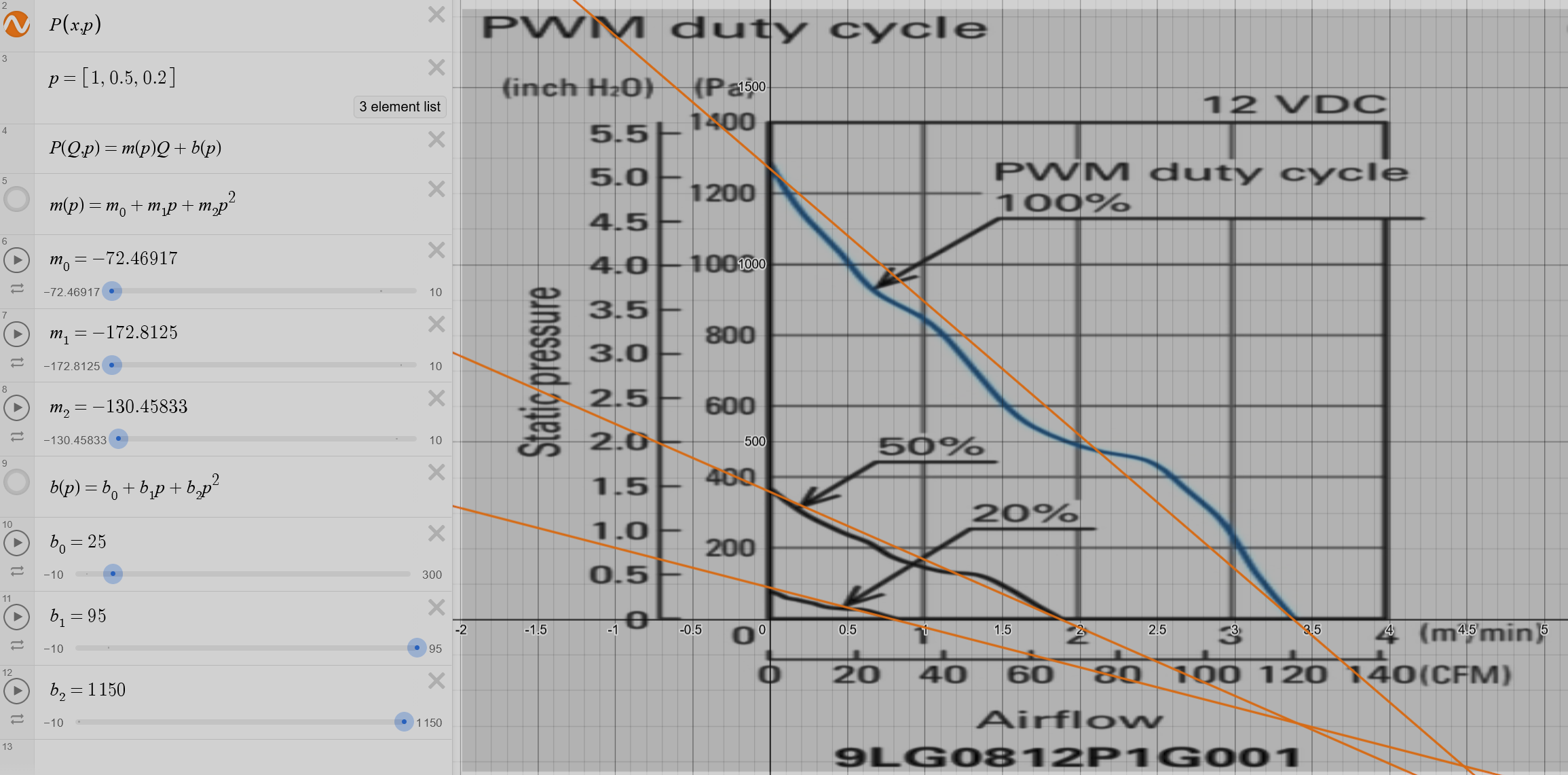

Online graphing used to interpolate manufacturer data from image
Source: Sanyo Denki 9GV Series Fan Datasheet

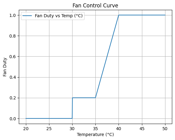
Temperature-Based Duty Control
#

A Fan duty cycle control law is defined piecewise based on battery temperature $t_K$ to optimize cooling. At lower temperatures, the fan is off or at minimum speed to save power. As temperature rises, the duty cycle ramps up linearly to maximum at a defined threshold.

# Kelvin thresholds
T_LOW_K = 273.15+30
T_MID_K = 273.15+35
DUTY_MIN = 0.20
DUTY_MAX = 1.00
# Ramp from 0.20 at 30°C to 1.0 at max_t_K
ramp_expr = DUTY_MIN + (t_K - T_MID_K) * (DUTY_MAX - DUTY_MIN)/(max_t_K - T_MID_K)
piecewise_expr = sp.Piecewise(
    (0, t_K <= T_LOW_K),
    (DUTY_MIN, t_K <= T_MID_K),  # 0.2
    (ramp_expr, sp.And(t_K > T_MID_K, t_K < max_t_K)),
    (DUTY_MAX, True)
)

fan_operating_curve = {
    "sympy_expr": piecewise_expr,
    "symbol": t_K,
    "params": {"max_t_K": max_t_K}
}

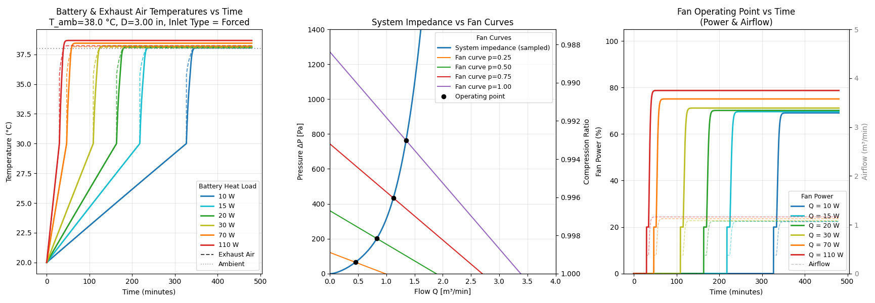
Operating Point Determination
#

The system finds equilibrium where fan curve intersects system impedance:

$$\Delta P_{fan}(Q) = \Delta P_{system}(Q)$$

Battery Pack Parameters
#

Parameter	Value	Source
Cell layout	36s8p (288 cells total)	Design Spec
Internal resistance	$14.5-15\,\mathrm{m\Omega}$	Datasheet
Pack Voltage	$130\,\mathrm{V}$	Design Spec
Pack Heat Output (Peak)	$110\,\mathrm{W}$	Internal Data
Thermal conductivity	$0.83 \frac{W}{m \cdot K}$	literature¹
Emissivity	0.65	literature²
Specific heat (per cell)	$C_{cell}(T_C) = 2.97 \cdot T_C + 907.5$ J/K (T_C in °C)	literature³

External Libraries
#

Library	Purpose	Notes
CoolProp	Thermophysical properties	Real gas EOS for air
SymPy	Symbolic fan curves	Enables parametric PWM control
NumPy	Numerical operations	Array math, interpolation
tubebank	Zukauskas correlations	Modified to fix interpolation bugs

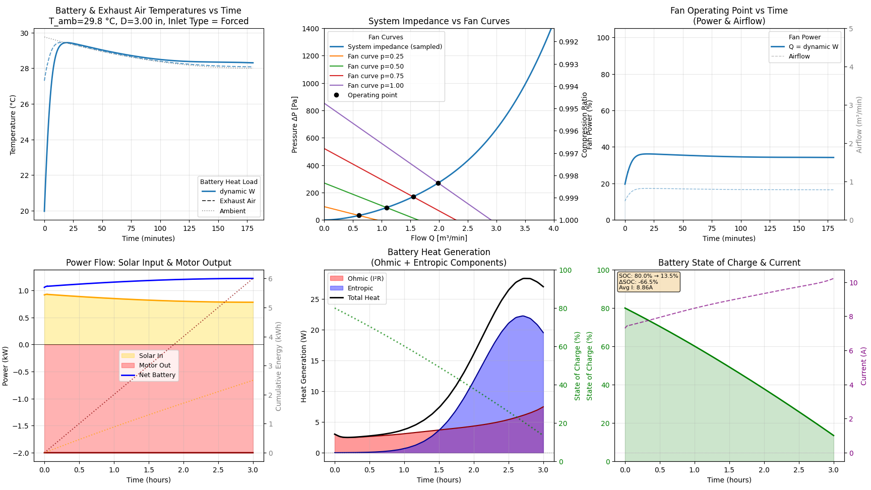
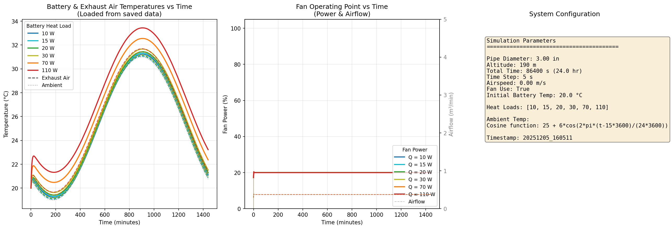
Key Results
#

The simulation produces:

Battery temperature vs. time for various heat loads
Fan operating point (duty cycle, flow rate) vs. time
System impedance curves with fan curve overlays
Steady-state temperatures at different power levels

System Impedance curves(center plot) help find the compression ratio of the system. This validates the incompressibile flow assumption used in fluid modeling.

The system can accurately model and track dynamic inputs (such as ambient temperature) for complex driving cycles and environmental conditions.

Code Quality Highlights
#

Caching: LRU cache on CoolProp calls with temperature/pressure quantization to avoid redundant lookups
Robust numerics: LMTD function handles edge cases (zero deltas, sign crossings, near-equal values)
Validation warnings: Biot number checks for lumped capacitance assumption validity
Modular design: Easy to swap components or add new correlation methods

@staticmethod
def air_props(T_K, p_Pa=None, h=0):
    # Quantized + cached with lru_cache to avoid redundant PropsSI calls.
    T_STEP = 0.1   # K
    P_STEP = 5.0   # Pa

    if p_Pa is None:
        p_Pa = CoolingComponent.P0 * math.exp(-CoolingComponent.g * h / (CoolingComponent.R * T_K))

    # quantize inputs
    T_bin = int(T_K // T_STEP * T_STEP)  # floor to lower step
    P_bin = int(p_Pa // P_STEP * P_STEP)  # floor to lower step

    return CoolingComponent._air_props_cached(T_bin, P_bin)

@staticmethod
@lru_cache(maxsize=4096)
def _air_props_cached(T_K_q, P_Pa_q):
    # Cached version of air_props
    rho = PropsSI("D", "T", T_K_q, "P", P_Pa_q, CoolingComponent.fluid) # density, kg/m^3
    mu = PropsSI("V", "T", T_K_q, "P", P_Pa_q, CoolingComponent.fluid) # dynamic viscosity, Pa.s
    k = PropsSI("L", "T", T_K_q, "P", P_Pa_q, CoolingComponent.fluid) # thermal conductivity, W/m-K
    Cp = PropsSI("C", "T", T_K_q, "P", P_Pa_q, CoolingComponent.fluid) # specific heat, J/kg-K

    Pr = PropsSI("PRANDTL", "T", T_K_q, "P", P_Pa_q, CoolingComponent.fluid) # Prandtl number, dimensionless
    gamma_cp = PropsSI("Cpmass", "T", T_K_q, "P", P_Pa_q, CoolingComponent.fluid) # Cp, J/kg-K
    gamma_cv = PropsSI("Cvmass", "T", T_K_q, "P", P_Pa_q, CoolingComponent.fluid) # Cv, J/kg-K
    gamma = gamma_cp / gamma_cv

    return {"rho": rho, "mu": mu, "k": k, "Cp": Cp, "Pr": Pr, "p": P_Pa_q, "gamma": gamma}

Data quantization and caching reduces expensive CoolProp calls significantly during time-stepping

2206 ms - WARNING - ThermalLoad: Mild Internal Gradients! Bi = 0.203
2572 ms - INFO - ThermalLoad: Biot Number Summary over 5760 steps:
2572 ms - INFO -   Max Bi = 0.370
2572 ms - INFO -   Mild (0.1-0.5):         3145 steps (54.6%)
2580 ms - INFO -   Significant (0.5-1.0):     0 steps (0.0%)
2580 ms - INFO -   Severe (>=1.0):            0 steps (0.0%)
2580 ms - INFO - Completed run for 15W heat load!
2581 ms - INFO - Fan energy used: 98.94 Wh over 8.00 hours
2581 ms - INFO - Running simulation for 20W heat load...
2686 ms - WARNING - ThermalLoad: Mild Internal Gradients! Bi = 0.203
3289 ms - INFO - ThermalLoad: Biot Number Summary over 5760 steps:
3289 ms - INFO -   Max Bi = 0.371
3289 ms - INFO -   Mild (0.1-0.5):         3798 steps (65.9%)
3289 ms - INFO -   Significant (0.5-1.0):     0 steps (0.0%)
3289 ms - INFO -   Severe (>=1.0):            0 steps (0.0%)
3289 ms - INFO - Completed run for 20W heat load!

Biot number warnings confirm the validity of the lumped capacity assumption of battery thermal model

Future Work
#

Transition off SymPy symbolic math for performance
Migrate to a more robust Heat Exchanger library like HT, implementing ESDU 73031
Refine Battery thermal model with more accurate geometry and conduction paths
Integrate with vehicle-level simulation for co-simulation of electrical and thermal systems

Results
#

Numerically quantified choices of Fans and Cooling Configurations for optimal battery temperatures
Created integral part of the vehicle simulation toolchain for Artemis 2026 and future solar cars

Key Skills
#

Programming: Python, OOP, Numerical Methods, Data Analysis
Fluids: Thermal Modeling, Heat Transfer, Fluid Dynamics
Simulation: Vehicle-level co-simulation, Battery thermal modeling

Overview#

Key Features#

System Architecture#

Physics & Equations#

Governing Energy Balance#

Convective Heat Transfer#

Log-Mean Temperature Difference#

Pressure Drop#

Darcy-Weisbach for tubes#

Zukauskas for tube banks#

Fan Control System#

PWM-Based Pressure Curve#

Temperature-Based Duty Control#

Operating Point Determination#

Battery Pack Parameters#

External Libraries#

Key Results#

Code Quality Highlights#

Future Work#

Results#

Key Skills#